A deep dive into Manim’s internals¶
Author: Benjamin Hackl
Disclaimer
This guide reflects the state of the library as of version v0.16.0
and primarily treats the Cairo renderer. The situation in the latest
version of Manim might be different; in case of substantial deviations
we will add a note below.
Introduction¶
Manim can be a wonderful library, if it behaves the way you would like it to, and/or the way you expect it to. Unfortunately, this is not always the case (as you probably know if you have played with some manimations yourself already). To understand where things go wrong, digging through the library’s source code is sometimes the only option – but in order to do that, you need to know where to start digging.
This article is intended as some sort of life line through the render process. We aim to give an appropriate amount of detail describing what happens when Manim reads your scene code and produces the corresponding animation. Throughout this article, we will focus on the following toy example:
from manim import *

class ToyExample(Scene):
    def construct(self):
        orange_square = Square(color=ORANGE, fill_opacity=0.5)
        blue_circle = Circle(color=BLUE, fill_opacity=0.5)
        self.add(orange_square)
        self.play(ReplacementTransform(orange_square, blue_circle, run_time=3))
        small_dot = Dot()
        small_dot.add_updater(lambda mob: mob.next_to(blue_circle, DOWN))
        self.play(Create(small_dot))
        self.play(blue_circle.animate.shift(RIGHT))
        self.wait()
        self.play(FadeOut(blue_circle, small_dot))
Before we go into details or even look at the rendered output of this scene,
let us first describe verbally what happens in this manimation. In the first
three lines of the construct method, a Square and a Circle
are initialized, then the square is added to the scene. The first frame of the
rendered output should thus show an orange square.
Then the actual animations happen: the square first transforms into a circle,
then a Dot is created (Where do you guess the dot is located when
it is first added to the scene? Answering this already requires detailed
knowledge about the render process.). The dot has an updater attached to it, and
as the circle moves right, the dot moves with it. In the end, all mobjects are
faded out.
Actually rendering the code yields the following video:
For this example, the output (fortunately) coincides with our expectations.
Overview¶
Because there is a lot of information in this article, here is a brief overview discussing the contents of the following chapters on a very high level.
Preliminaries: In this chapter we unravel all the steps that take place to prepare a scene for rendering; right until the point where the user-overridden
constructmethod is ran. This includes a brief discussion on using Manim’s CLI versus other means of rendering (e.g., via Jupyter notebooks, or in your Python script by calling theScene.render()method yourself).Mobject Initialization: For the second chapter we dive into creating and handling Mobjects, the basic elements that should be displayed in our scene. We discuss the
Mobjectbase class, how there are essentially three different types of Mobjects, and then discuss the most important of them, vectorized Mobjects. In particular, we describe the internal point data structure that governs how the mechanism responsible for drawing the vectorized Mobject to the screen sets the corresponding Bézier curves. We conclude the chapter with a tour intoScene.add(), the bookkeeping mechanism controlling which mobjects should be rendered.Animations and the Render Loop: And finally, in the last chapter we walk through the instantiation of
Animationobjects (the blueprints that hold information on how Mobjects should be modified when the render loop runs), followed by a investigation of the infamousScene.play()call. We will see that there are three relevant parts in aScene.play()call; a part in which the passed animations and keyword arguments are processed and prepared, followed by the actual “render loop” in which the library steps through a time line and renders frame by frame. The final part does some post-processing to save a short video segment (“partial movie file”) and cleanup for the next call toScene.play(). In the end, after all ofScene.construct()has been run, the library combines the partial movie files to one video.
And with that, let us get in medias res.
Preliminaries¶
Importing the library¶
Independent of how exactly you are telling your system
to render the scene, i.e., whether you run manim -qm -p file_name.py ToyExample, or
whether you are rendering the scene directly from the Python script via a snippet
like
with tempconfig({"quality": "medium_quality", "preview": True}):
    scene = ToyExample()
    scene.render()
or whether you are rendering the code in a Jupyter notebook, you are still telling your python interpreter to import the library. The usual pattern used to do this is
from manim import *
which (while being a debatable strategy in general) imports a lot of classes and
functions shipped with the library and makes them available in your global name space.
I explicitly avoided stating that it imports all classes and functions of the
library, because it does not do that: Manim makes use of the practice described
in Section 6.4.1 of the Python tutorial,
and all module members that should be exposed to the user upon running the *-import
are explicitly declared in the __all__ variable of the module.
Manim also uses this strategy internally: taking a peek at the file that is run when
the import is called, __init__.py (see
here),
you will notice that most of the code in that module is concerned with importing
members from various different submodules, again using *-imports.
Hint
If you would ever contribute a new submodule to Manim, the main
__init__.py is where it would have to be listed in order to make its
members accessible to users after importing the library.
In that file, there is one particular import at the beginning of the file however, namely:
from ._config import *
This initializes Manim’s global configuration system, which is used in various places
throughout the library. After the library runs this line, the current configuration
options are set. The code in there takes care of reading the options in your .cfg
files (all users have at least the global one that is shipped with the library)
as well as correctly handling command line arguments (if you used the CLI to render).
You can read more about the config system in the corresponding thematic guide, and if you are interested in learning more about the internals of the configuration system and how it is initialized, follow the code flow starting in the config module’s init file.
Now that the library is imported, we can turn our attention to the next step:
reading your scene code (which is not particularly exciting, Python just creates
a new class ToyExample based on our code; Manim is virtually not involved
in that step, with the exception that ToyExample inherits from Scene).
However, with the ToyExample class created and ready to go, there is a new
excellent question to answer: how is the code in our construct method
actually executed?
Scene instantiation and rendering¶
The answer to this question depends on how exactly you are running the code.
To make things a bit clearer, let us first consider the case that you
have created a file toy_example.py which looks like this:
from manim import *

class ToyExample(Scene):
    def construct(self):
        orange_square = Square(color=ORANGE, fill_opacity=0.5)
        blue_circle = Circle(color=BLUE, fill_opacity=0.5)
        self.add(orange_square)
        self.play(ReplacementTransform(orange_square, blue_circle, run_time=3))
        small_dot = Dot()
        small_dot.add_updater(lambda mob: mob.next_to(blue_circle, DOWN))
        self.play(Create(small_dot))
        self.play(blue_circle.animate.shift(RIGHT))
        self.wait()
        self.play(FadeOut(blue_circle, small_dot))

with tempconfig({"quality": "medium_quality", "preview": True}):
    scene = ToyExample()
    scene.render()
With such a file, the desired scene is rendered by simply running this Python
script via python toy_example.py. Then, as described above, the library
is imported and Python has read and defined the ToyExample class (but,
read carefully: no instance of this class has been created yet).
At this point, the interpreter is about to enter the tempconfig context
manager. Even if you have not seen Manim’s tempconfig before, its name
already suggests what it does: it creates a copy of the current state of the
configuration, applies the changes to the key-value pairs in the passed
dictionary, and upon leaving the context the original version of the
configuration is restored. TL;DR: it provides a fancy way of temporarily setting
configuration options.
Inside the context manager, two things happen: an actual ToyExample-scene
object is instantiated, and the render method is called. Every way of using
Manim ultimately does something along of these lines, the library always instantiates
the scene object and then calls its render method. To illustrate that this
really is the case, let us briefly look at the two most common ways of rendering
scenes:
Command Line Interface. When using the CLI and running the command
manim -qm -p toy_example.py ToyExample in your terminal, the actual
entry point is Manim’s __main__.py file (located
here.
Manim uses Click to implement
the command line interface, and the corresponding code is located in Manim’s
cli module (https://github.com/ManimCommunity/manim/tree/main/manim/cli).
The corresponding code creating the scene class and calling its render method
is located here.
Jupyter notebooks. In Jupyter notebooks, the communication with the library
is handled by the %%manim magic command, which is implemented in the
manim.utils.ipython_magic module. There is
some documentation available for the magic command,
and the code creating the scene class and calling its render method is located
here.
Now that we know that either way, a Scene object is created, let us investigate
what Manim does when that happens. When instantiating our scene object
scene = ToyExample()
the Scene.__init__ method is called, given that we did not implement our own initialization
method. Inspecting the corresponding code (see
here)
reveals that Scene.__init__ first sets several attributes of the scene objects that do not
depend on any configuration options set in config. Then the scene inspects the value of
config.renderer, and based on its value, either instantiates a CairoRenderer or an
OpenGLRenderer object and assigns it to its renderer attribute.
The scene then asks its renderer to initialize the scene by calling
self.renderer.init_scene(self)
Inspecting both the default Cairo renderer and the OpenGL renderer shows that the init_scene
method effectively makes the renderer instantiate a SceneFileWriter object, which
basically is Manim’s interface to libav (FFMPEG) and actually writes the movie file. The Cairo
renderer (see the implementation here) does not require any further initialization. The OpenGL renderer
does some additional setup to enable the realtime rendering preview window, which we do not go
into detail further here.
Warning
Currently, there is a lot of interplay between a scene and its renderer. This is a flaw in Manim’s current architecture, and we are working on reducing this interdependency to achieve a less convoluted code flow.
After the renderer has been instantiated and initialized its file writer, the scene populates
further initial attributes (notable mention: the mobjects attribute which keeps track
of the mobjects that have been added to the scene). It is then done with its instantiation
and ready to be rendered.
The rest of this article is concerned with the last line in our toy example script:
scene.render()
This is where the actual magic happens.
Inspecting the implementation of the render method
reveals that there are several hooks that can be used for pre- or postprocessing
a scene. Unsurprisingly, Scene.render() describes the full render cycle
of a scene. During this life cycle, there are three custom methods whose base
implementation is empty and that can be overwritten to suit your purposes. In
the order they are called, these customizable methods are:
Scene.setup(), which is intended for preparing and, well, setting up the scene for your animation (e.g., adding initial mobjects, assigning custom attributes to your scene class, etc.),Scene.construct(), which is the script for your screen play and contains programmatic descriptions of your animations, andScene.tear_down(), which is intended for any operations you might want to run on the scene after the last frame has already been rendered (for example, this could run some code that generates a custom thumbnail for the video based on the state of the objects in the scene – this hook is more relevant for situations where Manim is used within other Python scripts).
After these three methods are run, the animations have been fully rendered,
and Manim calls CairoRenderer.scene_finished() to gracefully
complete the rendering process. This checks whether any animations have been
played – and if so, it tells the SceneFileWriter to close the output
file. If not, Manim assumes that a static image should be output
which it then renders using the same strategy by calling the render loop
(see below) once.
Back in our toy example, the call to Scene.render() first
triggers Scene.setup() (which only consists of pass), followed by
a call of Scene.construct(). At this point, our animation script
is run, starting with the initialization of orange_square.
Mobject Initialization¶
Mobjects are, in a nutshell, the Python objects that represent all the things we want to display in our scene. Before we follow our debugger into the depths of mobject initialization code, it makes sense to discuss Manim’s different types of Mobjects and their basic data structure.
What even is a Mobject?¶
Mobject stands for mathematical object or Manim object
(depends on who you ask 😄). The Python class Mobject is
the base class for all objects that should be displayed on screen.
Looking at the initialization method
of Mobject, you will find that not too much happens in there:
some initial attribute values are assigned, like
name(which makes the render logs mention the name of the mobject instead of its type),submobjects(initially an empty list),color, and some others.Then, two methods related to points are called:
reset_pointsfollowed bygenerate_points,and finally,
init_colorsis called.
Digging deeper, you will find that Mobject.reset_points() simply
sets the points attribute of the mobject to an empty NumPy vector,
while the other two methods, Mobject.generate_points() and
Mobject.init_colors() are just implemented as pass.
This makes sense: Mobject is not supposed to be used as
an actual object that is displayed on screen; in fact the camera
(which we will discuss later in more detail; it is the class that is,
for the Cairo renderer, responsible for “taking a picture” of the
current scene) does not process “pure” Mobjects
in any way, they cannot even appear in the rendered output.
This is where different types of mobjects come into play. Roughly speaking, the Cairo renderer setup knows three different types of mobjects that can be rendered:
ImageMobject, which represent images that you can display in your scene,PMobject, which are very special mobjects used to represent point clouds; we will not discuss them further in this guide,VMobject, which are vectorized mobjects, that is, mobjects that consist of points that are connected via curves. These are pretty much everywhere, and we will discuss them in detail in the next section.
… and what are VMobjects?¶
As just mentioned, VMobjects represent vectorized
mobjects. To render a VMobject, the camera looks at the
points attribute of a VMobject and divides it into sets
of four points each. Each of these sets is then used to construct a
cubic Bézier curve with the first and last entry describing the
end points of the curve (“anchors”), and the second and third entry
describing the control points in between (“handles”).
Hint
To learn more about Bézier curves, take a look at the excellent online textbook A Primer on Bézier curves by Pomax – there is a playground representing cubic Bézier curves in §1, the red and yellow points are “anchors”, and the green and blue points are “handles”.
In contrast to Mobject, VMobject can be displayed
on screen (even though, technically, it is still considered a base class).
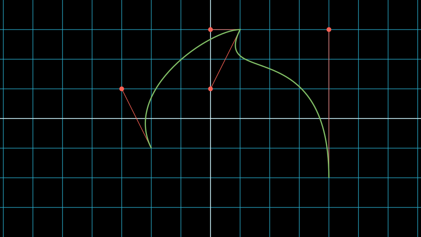
To illustrate how points are processed, consider the following short example
of a VMobject with 8 points (and thus made out of 8/4 = 2 cubic
Bézier curves). The resulting VMobject is drawn in green.
The handles are drawn as red dots with a line to their closest anchor.
Example: VMobjectDemo ¶
from manim import *

class VMobjectDemo(Scene):
    def construct(self):
        plane = NumberPlane()
        my_vmobject = VMobject(color=GREEN)
        my_vmobject.points = [
            np.array([-2, -1, 0]),  # start of first curve
            np.array([-3, 1, 0]),
            np.array([0, 3, 0]),
            np.array([1, 3, 0]),  # end of first curve
            np.array([1, 3, 0]),  # start of second curve
            np.array([0, 1, 0]),
            np.array([4, 3, 0]),
            np.array([4, -2, 0]),  # end of second curve
        ]
        handles = [
            Dot(point, color=RED) for point in
            [[-3, 1, 0], [0, 3, 0], [0, 1, 0], [4, 3, 0]]
        ]
        handle_lines = [
            Line(
                my_vmobject.points[ind],
                my_vmobject.points[ind+1],
                color=RED,
                stroke_width=2
            ) for ind in range(0, len(my_vmobject.points), 2)
        ]
        self.add(plane, *handles, *handle_lines, my_vmobject)
Squares and Circles: back to our Toy Example¶
With a basic understanding of different types of mobjects,
and an idea of how vectorized mobjects are built we can now
come back to our toy example and the execution of the
Scene.construct() method. In the first two lines
of our animation script, the orange_square and the
blue_circle are initialized.
When creating the orange square by running
Square(color=ORANGE, fill_opacity=0.5)
the initialization method of Square,
Square.__init__, is called. Looking at the
implementation,
we can see that the side_length attribute of the square is set,
and then
super().__init__(height=side_length, width=side_length, **kwargs)
is called. This super call is the Python way of calling the
initialization function of the parent class. As Square
inherits from Rectangle, the next method called
is Rectangle.__init__. There, only the first three lines
are really relevant for us:
super().__init__(UR, UL, DL, DR, color=color, **kwargs)
self.stretch_to_fit_width(width)
self.stretch_to_fit_height(height)
First, the initialization function of the parent class of
Rectangle – Polygon – is called. The
four positional arguments passed are the four corners of
the polygon: UR is up right (and equal to UP + RIGHT),
UL is up left (and equal to UP + LEFT), and so forth.
Before we follow our debugger deeper, let us observe what
happens with the constructed polygon: the remaining two lines
stretch the polygon to fit the specified width and height
such that a rectangle with the desired measurements is created.
The initialization function of Polygon is particularly
simple, it only calls the initialization function of its parent
class, Polygram. There, we have almost reached the end
of the chain: Polygram inherits from VMobject,
whose initialization function mainly sets the values of some
attributes (quite similar to Mobject.__init__, but more specific
to the Bézier curves that make up the mobject).
After calling the initialization function of VMobject,
the constructor of Polygram also does something somewhat
odd: it sets the points (which, you might remember above, should
actually be set in a corresponding generate_points method
of Polygram).
Warning
In several instances, the implementation of mobjects does not really stick to all aspects of Manim’s interface. This is unfortunate, and increasing consistency is something that we actively work on. Help is welcome!
Without going too much into detail, Polygram sets its
points attribute via VMobject.start_new_path(),
VMobject.add_points_as_corners(), which take care of
setting the quadruples of anchors and handles appropriately.
After the points are set, Python continues to process the
call stack until it reaches the method that was first called;
the initialization method of Square. After this,
the square is initialized and assigned to the orange_square
variable.
The initialization of blue_circle is similar to the one of
orange_square, with the main difference being that the inheritance
chain of Circle is different. Let us briefly follow the trace
of the debugger:
The implementation of Circle.__init__() immediately calls
the initialization method of Arc, as a circle in Manim
is simply an arc with an angle of \(\tau = 2\pi\). When
initializing the arc, some basic attributes are set (like
Arc.radius, Arc.arc_center, Arc.start_angle, and
Arc.angle), and then the initialization method of its
parent class, TipableVMobject, is called (which is
a rather abstract base class for mobjects which a arrow tip can
be attached to). Note that in contrast to Polygram,
this class does not preemptively generate the points of the circle.
After that, things are less exciting: TipableVMobject again
sets some attributes relevant for adding arrow tips, and afterwards
passes to the initialization method of VMobject. From there,
Mobject is initialized and Mobject.generate_points()
is called, which actually runs the method implemented in
Arc.generate_points().
After both our orange_square and the blue_circle are initialized,
the square is actually added to the scene. The Scene.add() method
is actually doing a few interesting things, so it is worth to dig a bit
deeper in the next section.
Adding Mobjects to the Scene¶
The code in our construct method that is run next is
self.add(orange_square)
From a high-level point of view, Scene.add() adds the
orange_square to the list of mobjects that should be rendered,
which is stored in the mobjects attribute of the scene. However,
it does so in a very careful way to avoid the situation that a mobject
is being added to the scene more than once. At a first glance, this
sounds like a simple task – the problem is that Scene.mobjects
is not a “flat” list of mobjects, but a list of mobjects which
might contain mobjects themselves, and so on.
Stepping through the code in Scene.add(), we see that first
it is checked whether we are currently using the OpenGL renderer
(which we are not) – adding mobjects to the scene works slightly
different (and actually easier!) for the OpenGL renderer. Then, the
code branch for the Cairo renderer is entered and the list of so-called
foreground mobjects (which are rendered on top of all other mobjects)
is added to the list of passed mobjects. This is to ensure that the
foreground mobjects will stay above of the other mobjects, even after
adding the new ones. In our case, the list of foreground mobjects
is actually empty, and nothing changes.
Next, Scene.restructure_mobjects() is called with the list
of mobjects to be added as the to_remove argument, which might
sound odd at first. Practically, this ensures that mobjects are not
added twice, as mentioned above: if they were present in the scene
Scene.mobjects list before (even if they were contained as a
child of some other mobject), they are first removed from the list.
The way Scene.restructure_mobjects() works is rather aggressive:
It always operates on a given list of mobjects; in the add method
two different lists occur: the default one, Scene.mobjects (no extra
keyword argument is passed), and Scene.moving_mobjects (which we will
discuss later in more detail). It iterates through all of the members of
the list, and checks whether any of the mobjects passed in to_remove
are contained as children (in any nesting level). If so, their parent
mobject is deconstructed and their siblings are inserted directly
one level higher. Consider the following example:
>>> from manim import Scene, Square, Circle, Group
>>> test_scene = Scene()
>>> mob1 = Square()
>>> mob2 = Circle()
>>> mob_group = Group(mob1, mob2)
>>> test_scene.add(mob_group)
<manim.scene.scene.Scene object at ...>
>>> test_scene.mobjects
[Group]
>>> test_scene.restructure_mobjects(to_remove=[mob1])
<manim.scene.scene.Scene object at ...>
>>> test_scene.mobjects
[Circle]
Note that the group is disbanded and the circle moves into the
root layer of mobjects in test_scene.mobjects.
After the mobject list is “restructured”, the mobject to be added
are simply appended to Scene.mobjects. In our toy example,
the Scene.mobjects list is actually empty, so the
restructure_mobjects method does not actually do anything. The
orange_square is simply added to Scene.mobjects, and as
the aforementioned Scene.moving_mobjects list is, at this point,
also still empty, nothing happens and Scene.add() returns.
We will hear more about the moving_mobject list when we discuss
the render loop. Before we do that, let us look at the next line
of code in our toy example, which includes the initialization of
an animation class,
ReplacementTransform(orange_square, blue_circle, run_time=3)
Hence it is time to talk about Animation.
Animations and the Render Loop¶
Initializing animations¶
Before we follow the trace of the debugger, let us briefly discuss
the general structure of the (abstract) base class Animation.
An animation object holds all the information necessary for the renderer
to generate the corresponding frames. Animations (in the sense of
animation objects) in Manim are always tied to a specific mobject;
even in the case of AnimationGroup (which you should actually
think of as an animation on a group of mobjects rather than a group
of animations). Moreover, except for in a particular special case,
the run time of animations is also fixed and known beforehand.
The initialization of animations actually is not very exciting,
Animation.__init__() merely sets some attributes derived
from the passed keyword arguments and additionally ensures that
the Animation.starting_mobject and Animation.mobject
attributes are populated. Once the animation is played, the
starting_mobject attribute holds an unmodified copy of the
mobject the animation is attached to; during the initialization
it is set to a placeholder mobject. The mobject attribute
is set to the mobject the animation is attached to.
Animations have a few special methods which are called during the render loop:
Animation.begin(), which is called (as hinted by its name) at the beginning of every animation, so before the first frame is rendered. In it, all the required setup for the animation happens.Animation.finish()is the counterpart to thebeginmethod which is called at the end of the life cycle of the animation (after the last frame has been rendered).Animation.interpolate()is the method that updates the mobject attached to the animation to the corresponding animation completion percentage. For example, if in the render loop,some_animation.interpolate(0.5)is called, the attached mobject will be updated to the state where 50% of the animation are completed.
We will discuss details about these and some further animation methods
once we walk through the actual render loop. For now, we continue with
our toy example and the code that is run when initializing the
ReplacementTransform animation.
The initialization method of ReplacementTransform only
consists of a call to the constructor of its parent class,
Transform, with the additional keyword argument
replace_mobject_with_target_in_scene set to True.
Transform then sets attributes that control how the
points of the starting mobject are deformed into the points of
the target mobject, and then passes on to the initialization
method of Animation. Other basic properties of the
animation (like its run_time, the rate_func, etc.) are
processed there – and then the animation object is fully
initialized and ready to be played.
The play call: preparing to enter Manim’s render loop¶
We are finally there, the render loop is in our reach. Let us
walk through the code that is run when Scene.play() is called.
Hint
Recall that this article is specifically about the Cairo renderer. Up to here, things were more or less the same for the OpenGL renderer as well; while some base mobjects might be different, the control flow and lifecycle of mobjects is still more or less the same. There are more substantial differences when it comes to the rendering loop.
As you will see when inspecting the method, Scene.play() almost
immediately passes over to the play method of the renderer,
in our case CairoRenderer.play. The one thing Scene.play()
takes care of is the management of subcaptions that you might have
passed to it (see the the documentation of Scene.play() and
Scene.add_subcaption() for more information).
Warning
As has been said before, the communication between scene and renderer is not in a very clean state at this point, so the following paragraphs might be confusing if you don’t run a debugger and step through the code yourself a bit.
Inside CairoRenderer.play(), the renderer first checks whether
it may skip rendering of the current play call. This might happen, for example,
when -s is passed to the CLI (i.e., only the last frame should be rendered),
or when the -n flag is passed and the current play call is outside of the
specified render bounds. The “skipping status” is updated in form of the
call to CairoRenderer.update_skipping_status().
Next, the renderer asks the scene to process the animations in the play
call so that renderer obtains all of the information it needs. To
be more concrete, Scene.compile_animation_data() is called,
which then takes care of several things:
The method processes all animations and the keyword arguments passed to the initial
Scene.play()call. In particular, this means that it makes sure all arguments passed to the play call are actually animations (or.animatesyntax calls, which are also assembled to be actualAnimation-objects at that point). It also propagates any animation-related keyword arguments (likerun_time, orrate_func) passed toScene.playto each individual animation. The processed animations are then stored in theanimationsattribute of the scene (which the renderer later reads…).It adds all mobjects to which the animations that are played are bound to to the scene (provided the animation is not an mobject-introducing animation – for these, the addition to the scene happens later).
In case the played animation is a
Waitanimation (this is the case in aScene.wait()call), the method checks whether a static image should be rendered, or whether the render loop should be processed as usual (seeScene.should_update_mobjects()for the exact conditions, basically it checks whether there are any time-dependent updater functions and so on).Finally, the method determines the total run time of the play call (which at this point is computed as the maximum of the run times of the passed animations). This is stored in the
durationattribute of the scene.
After the animation data has been compiled by the scene, the renderer
continues to prepare for entering the render loop. It now checks the
skipping status which has been determined before. If the renderer can
skip this play call, it does so: it sets the current play call hash (which
we will get back to in a moment) to None and increases the time of the
renderer by the determined animation run time.
Otherwise, the renderer checks whether or not Manim’s caching system should
be used. The idea of the caching system is simple: for every play call, a
hash value is computed, which is then stored and upon re-rendering the scene,
the hash is generated again and checked against the stored value. If it is the
same, the cached output is reused, otherwise it is fully rerendered again.
We will not go into details of the caching system here; if you would like
to learn more, the get_hash_from_play_call() function in the
utils.hashing module is essentially the entry point to the caching
mechanism.
In the event that the animation has to be rendered, the renderer asks
its SceneFileWriter to open an output container. The process
is started by a call to libav and opens a container to which rendered
raw frames can be written. As long as the output is open, the container
can be accessed via the output_container attribute of the file writer.
With the writing process in place, the renderer then asks the scene
to “begin” the animations.
First, it literally begins all of the animations by calling their
setup methods (Animation._setup_scene(), Animation.begin()).
In doing so, the mobjects that are newly introduced by an animation
(like via Create etc.) are added to the scene. Furthermore, the
animation suspends updater functions being called on its mobject, and
it sets its mobject to the state that corresponds to the first frame
of the animation.
After this has happened for all animations in the current play call,
the Cairo renderer determines which of the scene’s mobjects can be
painted statically to the background, and which ones have to be
redrawn every frame. It does so by calling
Scene.get_moving_and_static_mobjects(), and the resulting
partition of mobjects is stored in the corresponding moving_mobjects
and static_mobjects attributes.
Note
The mechanism that determines static and moving mobjects is
specific for the Cairo renderer, the OpenGL renderer works differently.
Basically, moving mobjects are determined by checking whether they,
any of their children, or any of the mobjects “below” them (in the
sense of the order in which mobjects are processed in the scene)
either have an update function attached, or whether they appear
in one of the current animations. See the implementation of
Scene.get_moving_mobjects() for more details.
Up to this very point, we did not actually render any (partial)
image or movie files from the scene yet. This is, however, about to change.
Before we enter the render loop, let us briefly revisit our toy
example and discuss how the generic Scene.play() call
setup looks like there.
For the call that plays the ReplacementTransform, there
is no subcaption to be taken care of. The renderer then asks
the scene to compile the animation data: the passed argument
already is an animation (no additional preparations needed),
there is no need for processing any keyword arguments (as
we did not specify any additional ones to play). The
mobject bound to the animation, orange_square, is already
part of the scene (so again, no action taken). Finally, the run
time is extracted (3 seconds long) and stored in
Scene.duration. The renderer then checks whether it should
skip (it should not), then whether the animation is already
cached (it is not). The corresponding animation hash value is
determined and passed to the file writer, which then also calls
libav to start the writing process which waits for rendered
frames from the library.
The scene then begins the animation: for the
ReplacementTransform this means that the animation populates
all of its relevant animation attributes (i.e., compatible copies
of the starting and the target mobject so that it can safely interpolate
between the two).
The mechanism determining static and moving mobjects considers
all of the scenes mobjects (at this point only the
orange_square), and determines that the orange_square is
bound to an animation that is currently played. As a result,
the square is classified as a “moving mobject”.
Time to render some frames.
The render loop (for real this time)¶
As mentioned above, due to the mechanism that determines static and moving mobjects in the scene, the renderer knows which mobjects it can paint statically to the background of the scene. Practically, this means that it partially renders a scene (to produce a background image), and then when iterating through the time progression of the animation only the “moving mobjects” are re-painted on top of the static background.
The renderer calls CairoRenderer.save_static_frame_data(), which
first checks whether there are currently any static mobjects, and if there
are, it updates the frame (only with the static mobjects; more about how
exactly this works in a moment) and then saves a NumPy array representing
the rendered frame in the static_image attribute. In our toy example,
there are no static mobjects, and so the static_image attribute is
simply set to None.
Next, the renderer asks the scene whether the current animation is a “frozen frame” animation, which would mean that the renderer actually does not have to repaint the moving mobjects in every frame of the time progression. It can then just take the latest static frame, and display it throughout the animation.
Note
An animation is considered a “frozen frame” animation if only a
static Wait animation is played. See the description
of Scene.compile_animation_data() above, or the
implementation of Scene.should_update_mobjects() for
more details.
If this is not the case (just as in our toy example), the renderer
then calls the Scene.play_internal() method, which is the
integral part of the render loop (in which the library steps through
the time progression of the animation and renders the corresponding
frames).
Within Scene.play_internal(), the following steps are performed:
The scene determines the run time of the animations by calling
Scene.get_run_time(). This method basically takes the maximumrun_timeattribute of all of the animations passed to theScene.play()call.Then the time progression is constructed via the (internal)
Scene._get_animation_time_progression()method, which wraps the actualScene.get_time_progression()method. The time progression is atqdmprogress bar object for an iterator overnp.arange(0, run_time, 1 / config.frame_rate). In other words, the time progression holds the time stamps (relative to the current animations, so starting at 0 and ending at the total animation run time, with the step size determined by the render frame rate) of the timeline where a new animation frame should be rendered.Then the scene iterates over the time progression: for each time stamp
t,Scene.update_to_time()is called, which …… first computes the time passed since the last update (which might be 0, especially for the initial call) and references it as
dt,then (in the order in which the animations are passed to
Scene.play()) callsAnimation.update_mobjects()to trigger all updater functions that are attached to the respective animation except for the “main mobject” of the animation (that is, for example, forTransformthe unmodified copies of start and target mobject – seeAnimation.get_all_mobjects_to_update()for more details),then the relative time progression with respect to the current animation is computed (
alpha = t / animation.run_time), which is then used to update the state of the animation with a call toAnimation.interpolate().After all of the passed animations have been processed, the updater functions of all mobjects in the scene, all meshes, and finally those attached to the scene itself are run.
At this point, the internal (Python) state of all mobjects has been updated to match the currently processed timestamp. If rendering should not be skipped, then it is now time to take a picture!
Note
The update of the internal state (iteration over the time progression) happens
always once Scene.play_internal() is entered. This ensures that even
if frames do not need to be rendered (because, e.g., the -n CLI flag has
been passed, something has been cached, or because we might be in a Section
with skipped rendering), updater functions still run correctly, and the state
of the first frame that is rendered is kept consistent.
To render an image, the scene calls the corresponding method of its renderer,
CairoRenderer.render() and passes just the list of moving mobjects (remember,
the static mobjects are assumed to have already been painted statically to
the background of the scene). All of the hard work then happens when the renderer
updates its current frame via a call to CairoRenderer.update_frame():
First, the renderer prepares its Camera by checking whether the renderer
has a static_image different from None stored already. If so, it sets the
image as the background image of the camera via Camera.set_frame_to_background(),
and otherwise it just resets the camera via Camera.reset(). The camera is then
asked to capture the scene with a call to Camera.capture_mobjects().
Things get a bit technical here, and at some point it is more efficient to delve into the implementation – but here is a summary of what happens once the camera is asked to capture the scene:
First, a flat list of mobjects is created (so submobjects get extracted from their parents). This list is then processed in groups of the same type of mobjects (e.g., a batch of vectorized mobjects, followed by a batch of image mobjects, followed by more vectorized mobjects, etc. – in many cases there will just be one batch of vectorized mobjects).
Depending on the type of the currently processed batch, the camera uses dedicated display functions to convert the
MobjectPython object to a NumPy array stored in the camera’spixel_arrayattribute. The most important example in that context is the display function for vectorized mobjects,Camera.display_multiple_vectorized_mobjects(), or the more particular (in case you did not add a background image to yourVMobject),Camera.display_multiple_non_background_colored_vmobjects(). This method first gets the current Cairo context, and then, for every (vectorized) mobject in the batch, callsCamera.display_vectorized(). There, the actual background stroke, fill, and then stroke of the mobject is drawn onto the context. SeeCamera.apply_stroke()andCamera.set_cairo_context_color()for more details – but it does not get much deeper than that, in the latter method the actual Bézier curves determined by the points of the mobject are drawn; this is where the low-level interaction with Cairo happens.
After all batches have been processed, the camera has an image representation
of the Scene at the current time stamp in form of a NumPy array stored in its
pixel_array attribute. The renderer then takes this array and passes it to
its SceneFileWriter. This concludes one iteration of the render loop,
and once the time progression has been processed completely, a final bit
of cleanup is performed before the Scene.play_internal() call is completed.
A TL;DR for the render loop, in the context of our toy example, reads as follows:
The scene finds that a 3 second long animation (the
ReplacementTransformchanging the orange square to the blue circle) should be played. Given the requested medium render quality, the frame rate is 30 frames per second, and so the time progression with steps[0, 1/30, 2/30, ..., 89/30]is created.In the internal render loop, each of these time stamps is processed: there are no updater functions, so effectively the scene updates the state of the transformation animation to the desired time stamp (for example, at time stamp
t = 45/30, the animation is completed to a rate ofalpha = 0.5).Then the scene asks the renderer to do its job. The renderer asks its camera to capture the scene, the only mobject that needs to be processed at this point is the main mobject attached to the transformation; the camera converts the current state of the mobject to entries in a NumPy array. The renderer passes this array to the file writer.
At the end of the loop, 90 frames have been passed to the file writer.
Completing the render loop¶
The last few steps in the Scene.play_internal() call are not too
exciting: for every animation, the corresponding Animation.finish()
and Animation.clean_up_from_scene() methods are called.
Note
Note that as part of Animation.finish(), the Animation.interpolate()
method is called with an argument of 1.0 – you might have noticed already that
the last frame of an animation can sometimes be a bit off or incomplete.
This is by current design! The last frame rendered in the render loop (and displayed
for a duration of 1 / frame_rate seconds in the rendered video) corresponds to
the state of the animation 1 / frame_rate seconds before it ends. To display
the final frame as well in the video, we would need to append another 1 / frame_rate
seconds to the video – which would then mean that a 1 second rendered Manim video
would be slightly longer than 1 second. We decided against this at some point.
In the end, the time progression is closed (which completes the displayed progress bar)
in the terminal. With the closing of the time progression, the
Scene.play_internal() call is completed, and we return to the renderer,
which now orders the SceneFileWriter to close the output container that has
been opened for this animation: a partial movie file is written.
This pretty much concludes the walkthrough of a Scene.play call,
and actually there is not too much more to say for our toy example either: at
this point, a partial movie file that represents playing the
ReplacementTransform has been written. The initialization of
the Dot happens analogous to the initialization of blue_circle,
which has been discussed above. The Mobject.add_updater() call literally
just attaches a function to the updaters attribute of the small_dot. And
the remaining Scene.play() and Scene.wait() calls follow the
exact same procedure as discussed in the render loop section above; each such call
produces a corresponding partial movie file.
Once the Scene.construct() method has been fully processed (and thus all
of the corresponding partial movie files have been written), the
scene calls its cleanup method Scene.tear_down(), and then
asks its renderer to finish the scene. The renderer, in turn, asks
its scene file writer to wrap things up by calling SceneFileWriter.finish(),
which triggers the combination of the partial movie files into the final product.
And there you go! This is a more or less detailed description of how Manim works under the hood. While we did not discuss every single line of code in detail in this walkthrough, it should still give you a fairly good idea of how the general structural design of the library and at least the Cairo rendering flow in particular looks like.