bezier

Utility functions related to Bézier curves.

Functions

bezier(points: BezierPointsLike) → Callable[[float | ColVector], Point3D | Point3D_Array]

bezier(points: Sequence[Point3DLike_Array]) → Callable[[float | ColVector], Point3D_Array]

Classic implementation of a Bézier curve.

Parameters:

points (TypeAliasForwardRef('~manim.typing.Point3D_Array') | Sequence[TypeAliasForwardRef('~manim.typing.Point3D_Array')]) – \((d+1, 3)\)-shaped array of \(d+1\) control points defining a single Bézier curve of degree \(d\). Alternatively, for vectorization purposes, points can also be a \((d+1, M, 3)\)-shaped sequence of \(d+1\) arrays of \(M\) control points each, which define M Bézier curves instead.

Returns:

bezier_func – Function describing the Bézier curve. The behaviour of this function depends on the shape of points:

• If points was a \((d+1, 3)\) array representing a single Bézier curve, then bezier_func can receive either:

  • a float t, in which case it returns a single \((1, 3)\)-shaped Point3D representing the evaluation of the Bézier at t, or

  • an \((n, 1)\)-shaped ColVector containing \(n\) values to evaluate the Bézier curve at, returning instead an \((n, 3)\)-shaped Point3D_Array containing the points resulting from evaluating the Bézier at each of the \(n\) values.

  Warning

  If passing a vector of \(t\)-values to bezier_func, it must be a column vector/matrix of shape \((n, 1)\). Passing an 1D array of shape \((n,)\) is not supported and will result in undefined behaviour.

• If points was a \((d+1, M, 3)\) array describing \(M\) Bézier curves, then bezier_func can receive either:

  • a float t, in which case it returns an \((M, 3)\)-shaped Point3D_Array representing the evaluation of the \(M\) Bézier curves at the same value t, or

  • an \((M, 1)\)-shaped ColVector containing \(M\) values, such that the \(i\)-th Bézier curve defined by points is evaluated at the corresponding \(i\)-th value in t, returning again an \((M, 3)\)-shaped Point3D_Array containing those \(M\) evaluations.

  Warning

  Unlike the previous case, if you pass a ColVector to bezier_func, it must contain exactly \(M\) values, each value for each of the \(M\) Bézier curves defined by points. Any array of shape other than \((M, 1)\) will result in undefined behaviour.

Return type:

typing.Callable [[float | ColVector], Point3D | Point3D_Array]

bezier_remap(bezier_tuples, new_number_of_curves)

Subdivides each curve in bezier_tuples into as many parts as necessary, until the final number of curves reaches a desired amount, new_number_of_curves.

Parameters:

• bezier_tuples (BezierPointsLike_Array) –

  An array of multiple Bézier curves of degree \(d\) to be remapped. The shape of this array must be (current_number_of_curves, nppc, dim), where:

  • current_number_of_curves is the current amount of curves in the array bezier_tuples,

  • nppc is the amount of points per curve, such that their degree is nppc-1, and

  • dim is the dimension of the points, usually \(3\).

• new_number_of_curves (int) – The number of curves that the output will contain. This needs to be higher than the current number.

Returns:

The new array of shape (new_number_of_curves, nppc, dim), containing the new Bézier curves after the remap.

Return type:

BezierPoints_Array

get_quadratic_approximation_of_cubic(a0: Point3DLike, h0: Point3DLike, h1: Point3DLike, a1: Point3DLike) → QuadraticSpline

get_quadratic_approximation_of_cubic(a0: Point3DLike_Array, h0: Point3DLike_Array, h1: Point3DLike_Array, a1: Point3DLike_Array) → QuadraticBezierPath

If a0, h0, h1 and a1 are the control points of a cubic Bézier curve, approximate the curve with two quadratic Bézier curves and return an array of 6 points, where the first 3 points represent the first quadratic curve and the last 3 represent the second one.

Otherwise, if a0, h0, h1 and a1 are _arrays_ of \(N\) points representing \(N\) cubic Bézier curves, return an array of \(6N\) points where each group of \(6\) consecutive points approximates each of the \(N\) curves in a similar way as above.

Note

If the cubic spline given by the original cubic Bézier curves is smooth, this algorithm will generate a quadratic spline which is also smooth.

If a cubic Bézier is given by

\[C(t) = (1-t)^3 A_0 + 3(1-t)^2 t H_0 + 3(1-t)t^2 H_1 + t^3 A_1\]

where \(A_0\), \(H_0\), \(H_1\) and \(A_1\) are its control points, then this algorithm should generate two quadratic Béziers given by

\[\begin{split}Q_0(t) &= (1-t)^2 A_0 + 2(1-t)t M_0 + t^2 K \\ Q_1(t) &= (1-t)^2 K + 2(1-t)t M_1 + t^2 A_1\end{split}\]

where \(M_0\) and \(M_1\) are the respective handles to be found for both curves, and \(K\) is the end anchor of the 1st curve and the start anchor of the 2nd, which must also be found.

To solve for \(M_0\), \(M_1\) and \(K\), three conditions can be imposed:

1. \(Q_0'(0) = \frac{1}{2}C'(0)\). The derivative of the first quadratic curve at \(t = 0\) should be proportional to that of the original cubic curve, also at \(t = 0\). Because the cubic curve is split into two parts, it is necessary to divide this by two: the speed of a point travelling through the curve should be half of the original. This gives:

   \[\begin{split}Q_0'(0) &= \frac{1}{2}C'(0) \\ 2(M_0 - A_0) &= \frac{3}{2}(H_0 - A_0) \\ 2M_0 - 2A_0 &= \frac{3}{2}H_0 - \frac{3}{2}A_0 \\ 2M_0 &= \frac{3}{2}H_0 + \frac{1}{2}A_0 \\ M_0 &= \frac{1}{4}(3H_0 + A_0)\end{split}\]

2. \(Q_1'(1) = \frac{1}{2}C'(1)\). The derivative of the second quadratic curve at \(t = 1\) should be half of that of the original cubic curve for the same reasons as above, also at \(t = 1\). This gives:

   \[\begin{split}Q_1'(1) &= \frac{1}{2}C'(1) \\ 2(A_1 - M_1) &= \frac{3}{2}(A_1 - H_1) \\ 2A_1 - 2M_1 &= \frac{3}{2}A_1 - \frac{3}{2}H_1 \\ -2M_1 &= -\frac{1}{2}A_1 - \frac{3}{2}H_1 \\ M_1 &= \frac{1}{4}(3H_1 + A_1)\end{split}\]

3. \(Q_0'(1) = Q_1'(0)\). The derivatives of both quadratic curves should match at the point \(K\), in order for the final spline to be smooth. This gives:

   \[\begin{split}Q_0'(1) &= Q_1'(0) \\ 2(K - M_0) &= 2(M_1 - K) \\ 2K - 2M_0 &= 2M_1 - 2K \\ 4K &= 2M_0 + 2M_1 \\ K &= \frac{1}{2}(M_0 + M_1)\end{split}\]

This is sufficient to find proper control points for the quadratic Bézier curves.

Parameters:

• a0 (TypeAliasForwardRef('~manim.typing.Point3D') | TypeAliasForwardRef('~manim.typing.Point3D_Array')) – The start anchor of a single cubic Bézier curve, or an array of \(N\) start anchors for \(N\) curves.

• h0 (TypeAliasForwardRef('~manim.typing.Point3D') | TypeAliasForwardRef('~manim.typing.Point3D_Array')) – The first handle of a single cubic Bézier curve, or an array of \(N\) first handles for \(N\) curves.

• h1 (TypeAliasForwardRef('~manim.typing.Point3D') | TypeAliasForwardRef('~manim.typing.Point3D_Array')) – The second handle of a single cubic Bézier curve, or an array of \(N\) second handles for \(N\) curves.

• a1 (TypeAliasForwardRef('~manim.typing.Point3D') | TypeAliasForwardRef('~manim.typing.Point3D_Array')) – The end anchor of a single cubic Bézier curve, or an array of \(N\) end anchors for \(N\) curves.

Returns:

An array containing either 6 points for 2 quadratic Bézier curves approximating the original cubic curve, or \(6N\) points for \(2N\) quadratic curves approximating \(N\) cubic curves.

Return type:

result

Raises:

ValueError – If a0, h0, h1 and a1 have different dimensions, or if their number of dimensions is not 1 or 2.

get_smooth_closed_cubic_bezier_handle_points(anchors)

Special case of get_smooth_cubic_bezier_handle_points(), when the anchors form a closed loop.

Note

A system of equations must be solved to get the first handles of every Bézier curve (referred to as \(H_1\)). Then \(H_2\) (the second handles) can be obtained separately.

See also

The equations were obtained from:

• Conditions on control points for continuous curvature. (2016). Jaco Stuifbergen.

In general, if there are \(N+1\) anchors, there will be \(N\) Bézier curves and thus \(N\) pairs of handles to find. We must solve the following system of equations for the 1st handles (example for \(N = 5\)):

\[\begin{split}\begin{pmatrix} 4 & 1 & 0 & 0 & 1 \\ 1 & 4 & 1 & 0 & 0 \\ 0 & 1 & 4 & 1 & 0 \\ 0 & 0 & 1 & 4 & 1 \\ 1 & 0 & 0 & 1 & 4 \end{pmatrix} \begin{pmatrix} H_{1,0} \\ H_{1,1} \\ H_{1,2} \\ H_{1,3} \\ H_{1,4} \end{pmatrix} = \begin{pmatrix} 4A_0 + 2A_1 \\ 4A_1 + 2A_2 \\ 4A_2 + 2A_3 \\ 4A_3 + 2A_4 \\ 4A_4 + 2A_5 \end{pmatrix}\end{split}\]

which will be expressed as \(RH_1 = D\).

\(R\) is almost a tridiagonal matrix, so we could use Thomas’ algorithm.

See also

Tridiagonal matrix algorithm. Wikipedia.

However, \(R\) has ones at the opposite corners. A solution to this is the first decomposition proposed in the link below, with \(\alpha = 1\):

See also

Tridiagonal matrix algorithm # Variants. Wikipedia.

\[\begin{split}R = \begin{pmatrix} 4 & 1 & 0 & 0 & 1 \\ 1 & 4 & 1 & 0 & 0 \\ 0 & 1 & 4 & 1 & 0 \\ 0 & 0 & 1 & 4 & 1 \\ 1 & 0 & 0 & 1 & 4 \end{pmatrix} &= \begin{pmatrix} 3 & 1 & 0 & 0 & 0 \\ 1 & 4 & 1 & 0 & 0 \\ 0 & 1 & 4 & 1 & 0 \\ 0 & 0 & 1 & 4 & 1 \\ 0 & 0 & 0 & 1 & 3 \end{pmatrix} + \begin{pmatrix} 1 & 0 & 0 & 0 & 1 \\ 0 & 0 & 0 & 0 & 0 \\ 0 & 0 & 0 & 0 & 0 \\ 0 & 0 & 0 & 0 & 0 \\ 1 & 0 & 0 & 0 & 1 \end{pmatrix} \\ & \\ &= \begin{pmatrix} 3 & 1 & 0 & 0 & 0 \\ 1 & 4 & 1 & 0 & 0 \\ 0 & 1 & 4 & 1 & 0 \\ 0 & 0 & 1 & 4 & 1 \\ 0 & 0 & 0 & 1 & 3 \end{pmatrix} + \begin{pmatrix} 1 \\ 0 \\ 0 \\ 0 \\ 1 \end{pmatrix} \begin{pmatrix} 1 & 0 & 0 & 0 & 1 \end{pmatrix} \\ & \\ &= T + uv^t\end{split}\]

We decompose \(R = T + uv^t\), where \(T\) is a tridiagonal matrix, and \(u, v\) are \(N\)-D vectors such that \(u_0 = u_{N-1} = v_0 = v_{N-1} = 1\), and \(u_i = v_i = 0, \forall i \in \{1, ..., N-2\}\).

Thus:

\[\begin{split}RH_1 &= D \\ \Rightarrow (T + uv^t)H_1 &= D\end{split}\]

If we find a vector \(q\) such that \(Tq = u\):

\[\begin{split}\Rightarrow (T + Tqv^t)H_1 &= D \\ \Rightarrow T(I + qv^t)H_1 &= D \\ \Rightarrow H_1 &= (I + qv^t)^{-1} T^{-1} D\end{split}\]

According to Sherman-Morrison’s formula:

See also

Sherman-Morrison’s formula. Wikipedia.

\[(I + qv^t)^{-1} = I - \frac{1}{1 + v^tq} qv^t\]

If we find \(Y = T^{-1} D\), or in other words, if we solve for \(Y\) in \(TY = D\):

\[\begin{split}H_1 &= (I + qv^t)^{-1} T^{-1} D \\ &= (I + qv^t)^{-1} Y \\ &= (I - \frac{1}{1 + v^tq} qv^t) Y \\ &= Y - \frac{1}{1 + v^tq} qv^tY\end{split}\]

Therefore, we must solve for \(q\) and \(Y\) in \(Tq = u\) and \(TY = D\). As \(T\) is now tridiagonal, we shall use Thomas’ algorithm.

Define:

• \(a = [a_0, \ a_1, \ ..., \ a_{N-2}]\) as \(T\)’s lower diagonal of \(N-1\) elements, such that \(a_0 = a_1 = ... = a_{N-2} = 1\), so this diagonal is filled with ones;

• \(b = [b_0, \ b_1, \ ..., \ b_{N-2}, \ b_{N-1}]\) as \(T\)’s main diagonal of \(N\) elements, such that \(b_0 = b_{N-1} = 3\), and \(b_1 = b_2 = ... = b_{N-2} = 4\);

• \(c = [c_0, \ c_1, \ ..., \ c_{N-2}]\) as \(T\)’s upper diagonal of \(N-1\) elements, such that \(c_0 = c_1 = ... = c_{N-2} = 1\): this diagonal is also filled with ones.

If, according to Thomas’ algorithm, we define:

\[\begin{split}c'_0 &= \frac{c_0}{b_0} & \\ c'_i &= \frac{c_i}{b_i - a_{i-1} c'_{i-1}}, & \quad \forall i \in \{1, ..., N-2\} \\ & & \\ u'_0 &= \frac{u_0}{b_0} & \\ u'_i &= \frac{u_i - a_{i-1} u'_{i-1}}{b_i - a_{i-1} c'_{i-1}}, & \quad \forall i \in \{1, ..., N-1\} \\ & & \\ D'_0 &= \frac{1}{b_0} D_0 & \\ D'_i &= \frac{1}{b_i - a_{i-1} c'_{i-1}} (D_i - a_{i-1} D'_{i-1}), & \quad \forall i \in \{1, ..., N-1\}\end{split}\]

Then:

\[\begin{split}c'_0 &= \frac{1}{3} & \\ c'_i &= \frac{1}{4 - c'_{i-1}}, & \quad \forall i \in \{1, ..., N-2\} \\ & & \\ u'_0 &= \frac{1}{3} & \\ u'_i &= \frac{-u'_{i-1}}{4 - c'_{i-1}} = -c'_i u'_{i-1}, & \quad \forall i \in \{1, ..., N-2\} \\ u'_{N-1} &= \frac{1 - u'_{N-2}}{3 - c'_{N-2}} & \\ & & \\ D'_0 &= \frac{1}{3} (4A_0 + 2A_1) & \\ D'_i &= \frac{1}{4 - c'_{i-1}} (4A_i + 2A_{i+1} - D'_{i-1}) & \\ &= c_i (4A_i + 2A_{i+1} - D'_{i-1}), & \quad \forall i \in \{1, ..., N-2\} \\ D'_{N-1} &= \frac{1}{3 - c'_{N-2}} (4A_{N-1} + 2A_N - D'_{N-2}) &\end{split}\]

Finally, we can do Backward Substitution to find \(q\) and \(Y\):

\[\begin{split}q_{N-1} &= u'_{N-1} & \\ q_i &= u'_{i} - c'_i q_{i+1}, & \quad \forall i \in \{0, ..., N-2\} \\ & & \\ Y_{N-1} &= D'_{N-1} & \\ Y_i &= D'_i - c'_i Y_{i+1}, & \quad \forall i \in \{0, ..., N-2\}\end{split}\]

With those values, we can finally calculate \(H_1 = Y - \frac{1}{1 + v^tq} qv^tY\). Given that \(v_0 = v_{N-1} = 1\), and \(v_1 = v_2 = ... = v_{N-2} = 0\), its dot products with \(q\) and \(Y\) are respectively \(v^tq = q_0 + q_{N-1}\) and \(v^tY = Y_0 + Y_{N-1}\). Thus:

\[H_1 = Y - \frac{1}{1 + q_0 + q_{N-1}} q(Y_0 + Y_{N-1})\]

Once we have \(H_1\), we can get \(H_2\) (the array of second handles) as follows:

\[\begin{split}H_{2, i} &= 2A_{i+1} - H_{1, i+1}, & \quad \forall i \in \{0, ..., N-2\} \\ H_{2, N-1} &= 2A_0 - H_{1, 0} &\end{split}\]

Because the matrix \(R\) always follows the same pattern (and thus \(T, u, v\) as well), we can define a memo list for \(c'\) and \(u'\) to avoid recalculation. We cannot memoize \(D\) and \(Y\), however, because they are always different matrices. We cannot make a memo for \(q\) either, but we can calculate it faster because \(u'\) can be memoized.

Parameters:

anchors (Point3DLike_Array) – Anchors of a closed cubic spline.

Returns:

A tuple of two arrays: one containing the 1st handle for every curve in the closed cubic spline, and the other containing the 2nd handles.

Return type:

tuple [Point3D_Array, Point3D_Array]

get_smooth_cubic_bezier_handle_points(anchors)

Given an array of anchors for a cubic spline (array of connected cubic Bézier curves), compute the 1st and 2nd handle for every curve, so that the resulting spline is smooth.

Parameters:

anchors (Point3DLike_Array) – Anchors of a cubic spline.

Returns:

A tuple of two arrays: one containing the 1st handle for every curve in the cubic spline, and the other containing the 2nd handles.

Return type:

tuple [Point3D_Array, Point3D_Array]

get_smooth_open_cubic_bezier_handle_points(anchors)

Special case of get_smooth_cubic_bezier_handle_points(), when the anchors do not form a closed loop.

Note

A system of equations must be solved to get the first handles of every Bèzier curve (referred to as \(H_1\)). Then \(H_2\) (the second handles) can be obtained separately.

See also

The equations were obtained from:

• Smooth Bézier Spline Through Prescribed Points. (2012). Particle in Cell Consulting LLC.

• Conditions on control points for continuous curvature. (2016). Jaco Stuifbergen.

Warning

The equations in the first webpage have some typos which were corrected in the comments.

In general, if there are \(N+1\) anchors, there will be \(N\) Bézier curves and thus \(N\) pairs of handles to find. We must solve the following system of equations for the 1st handles (example for \(N = 5\)):

\[\begin{split}\begin{pmatrix} 2 & 1 & 0 & 0 & 0 \\ 1 & 4 & 1 & 0 & 0 \\ 0 & 1 & 4 & 1 & 0 \\ 0 & 0 & 1 & 4 & 1 \\ 0 & 0 & 0 & 2 & 7 \end{pmatrix} \begin{pmatrix} H_{1,0} \\ H_{1,1} \\ H_{1,2} \\ H_{1,3} \\ H_{1,4} \end{pmatrix} = \begin{pmatrix} A_0 + 2A_1 \\ 4A_1 + 2A_2 \\ 4A_2 + 2A_3 \\ 4A_3 + 2A_4 \\ 8A_4 + A_5 \end{pmatrix}\end{split}\]

which will be expressed as \(TH_1 = D\). \(T\) is a tridiagonal matrix, so the system can be solved in \(O(N)\) operations. Here we shall use Thomas’ algorithm or the tridiagonal matrix algorithm.

See also

Tridiagonal matrix algorithm. Wikipedia.

Define:

• \(a = [a_0, \ a_1, \ ..., \ a_{N-2}]\) as \(T\)’s lower diagonal of \(N-1\) elements, such that \(a_0 = a_1 = ... = a_{N-3} = 1\), and \(a_{N-2} = 2\);

• \(b = [b_0, \ b_1, \ ..., \ b_{N-2}, \ b_{N-1}]\) as \(T\)’s main diagonal of \(N\) elements, such that \(b_0 = 2\), \(b_1 = b_2 = ... = b_{N-2} = 4\), and \(b_{N-1} = 7\);

• \(c = [c_0, \ c_1, \ ..., \ c_{N-2}]\) as \(T\)’s upper diagonal of \({N-1}\) elements, such that \(c_0 = c_1 = ... = c_{N-2} = 1\): this diagonal is filled with ones.

If, according to Thomas’ algorithm, we define:

\[\begin{split}c'_0 &= \frac{c_0}{b_0} & \\ c'_i &= \frac{c_i}{b_i - a_{i-1} c'_{i-1}}, & \quad \forall i \in \{1, ..., N-2\} \\ & & \\ D'_0 &= \frac{1}{b_0} D_0 & \\ D'_i &= \frac{1}{b_i - a_{i-1} c'{i-1}} (D_i - a_{i-1} D'_{i-1}), & \quad \forall i \in \{1, ..., N-1\}\end{split}\]

Then:

\[\begin{split}c'_0 &= 0.5 & \\ c'_i &= \frac{1}{4 - c'_{i-1}}, & \quad \forall i \in \{1, ..., N-2\} \\ & & \\ D'_0 &= 0.5A_0 + A_1 & \\ D'_i &= \frac{1}{4 - c'_{i-1}} (4A_i + 2A_{i+1} - D'_{i-1}) & \\ &= c_i (4A_i + 2A_{i+1} - D'_{i-1}), & \quad \forall i \in \{1, ..., N-2\} \\ D'_{N-1} &= \frac{1}{7 - 2c'_{N-2}} (8A_{N-1} + A_N - 2D'_{N-2}) &\end{split}\]

Finally, we can do Backward Substitution to find \(H_1\):

\[\begin{split}H_{1, N-1} &= D'_{N-1} & \\ H_{1, i} &= D'_i - c'_i H_{1, i+1}, & \quad \forall i \in \{0, ..., N-2\}\end{split}\]

Once we have \(H_1\), we can get \(H_2\) (the array of second handles) as follows:

\[\begin{split}H_{2, i} &= 2A_{i+1} - H_{1, i+1}, & \quad \forall i \in \{0, ..., N-2\} \\ H_{2, N-1} &= 0.5A_N + 0.5H_{1, N-1} &\end{split}\]

As the matrix \(T\) always follows the same pattern, we can define a memo list for \(c'\) to avoid recalculation. We cannot do the same for \(D\), however, because it is always a different matrix.

Parameters:

anchors (Point3DLike_Array) – Anchors of an open cubic spline.

Returns:

A tuple of two arrays: one containing the 1st handle for every curve in the open cubic spline, and the other containing the 2nd handles.

Return type:

tuple [Point3D_Array, Point3D_Array]

integer_interpolate(start, end, alpha)

This is a variant of interpolate that returns an integer and the residual

Parameters:

• start (float) – The start of the range

• end (float) – The end of the range

• alpha (float) – a float between 0 and 1.

Returns:

This returns an integer between start and end (inclusive) representing appropriate interpolation between them, along with a “residue” representing a new proportion between the returned integer and the next one of the list.

Return type:

tuple[int, float]

Example

>>> integer, residue = integer_interpolate(start=0, end=10, alpha=0.46)
>>> np.allclose((integer, residue), (4, 0.6))
True

interpolate(start: float, end: float, alpha: float) → float

interpolate(start: float, end: float, alpha: ColVector) → ColVector

interpolate(start: Point3D, end: Point3D, alpha: float) → Point3D

interpolate(start: Point3D, end: Point3D, alpha: ColVector) → Point3D_Array

Linearly interpolates between two values start and end.

Parameters:

• start (float | TypeAliasForwardRef('~manim.typing.Point3D')) – The start of the range.

• end (float | TypeAliasForwardRef('~manim.typing.Point3D')) – The end of the range.

• alpha (float | TypeAliasForwardRef('~manim.typing.ColVector')) – A float between 0 and 1, or an \((n, 1)\) column vector containing \(n\) floats between 0 and 1 to interpolate in a vectorized fashion.

Returns:

The result of the linear interpolation.

• If start and end are of type float, and:

  • alpha is also a float, the return is simply another float.

  • alpha is a ColVector, the return is another ColVector.

• If start and end are of type Point3D, and:

  • alpha is a float, the return is another Point3D.

  • alpha is a ColVector, the return is a Point3D_Array.

Return type:

float | ColVector | Point3D | Point3D_Array

inverse_interpolate(start: float, end: float, value: float) → float

inverse_interpolate(start: float, end: float, value: Point3D) → Point3D

inverse_interpolate(start: Point3D, end: Point3D, value: Point3D) → Point3D

Perform inverse interpolation to determine the alpha values that would produce the specified value given the start and end values or points.

Parameters:

• start (float | TypeAliasForwardRef('~manim.typing.Point3D')) – The start value or point of the interpolation.

• end (float | TypeAliasForwardRef('~manim.typing.Point3D')) – The end value or point of the interpolation.

• value (float | TypeAliasForwardRef('~manim.typing.Point3D')) – The value or point for which the alpha value should be determined.

Returns:

• The alpha values producing the given input

• when interpolating between start and end.

Return type:

float | TypeAliasForwardRef(‘~manim.typing.Point3D’)

Example

>>> inverse_interpolate(start=2, end=6, value=4)
np.float64(0.5)

>>> start = np.array([1, 2, 1])
>>> end = np.array([7, 8, 11])
>>> value = np.array([4, 5, 5])
>>> inverse_interpolate(start, end, value)
array([0.5, 0.5, 0.4])

is_closed(points)

Returns True if the spline given by points is closed, by checking if its first and last points are close to each other, or``False`` otherwise.

Note

This function reimplements np.allclose(), because repeated calling of np.allclose() for only 2 points is inefficient.

Parameters:

points (Point3D_Array) – An array of points defining a spline.

Returns:

Whether the first and last points of the array are close enough or not to be considered the same, thus considering the defined spline as closed.

Return type:

bool

Examples

>>> import numpy as np
>>> from manim import is_closed
>>> is_closed(
...     np.array(
...         [
...             [0, 0, 0],
...             [1, 2, 3],
...             [3, 2, 1],
...             [0, 0, 0],
...         ]
...     )
... )
True
>>> is_closed(
...     np.array(
...         [
...             [0, 0, 0],
...             [1, 2, 3],
...             [3, 2, 1],
...             [1e-10, 1e-10, 1e-10],
...         ]
...     )
... )
True
>>> is_closed(
...     np.array(
...         [
...             [0, 0, 0],
...             [1, 2, 3],
...             [3, 2, 1],
...             [1e-2, 1e-2, 1e-2],
...         ]
...     )
... )
False

match_interpolate(new_start: float, new_end: float, old_start: float, old_end: float, old_value: float) → float

match_interpolate(new_start: float, new_end: float, old_start: float, old_end: float, old_value: Point3D) → Point3D

Interpolate a value from an old range to a new range.

Parameters:

• new_start (float) – The start of the new range.

• new_end (float) – The end of the new range.

• old_start (float) – The start of the old range.

• old_end (float) – The end of the old range.

• old_value (float | TypeAliasForwardRef('~manim.typing.Point3D')) – The value within the old range whose corresponding value in the new range (with the same alpha value) is desired.

Return type:

The interpolated value within the new range.

Examples

>>> from manim import match_interpolate
>>> match_interpolate(0, 100, 10, 20, 15)
np.float64(50.0)

mid(start: float, end: float) → float

mid(start: Point3D, end: Point3D) → Point3D

Returns the midpoint between two values.

Parameters:

• start (float | TypeAliasForwardRef('~manim.typing.Point3D')) – The first value

• end (float | TypeAliasForwardRef('~manim.typing.Point3D')) – The second value

Return type:

The midpoint between the two values

partial_bezier_points(points, a, b)

Given an array of points which define a Bézier curve, and two numbers \(a, b\) such that \(0 \le a < b \le 1\), return an array of the same size, which describes the portion of the original Bézier curve on the interval \([a, b]\).

partial_bezier_points() is conceptually equivalent to calling split_bezier() twice and discarding unused Bézier curves, but this is more efficient and doesn’t waste computations.

See also

See split_bezier() for an explanation on how to split Bézier curves.

Note

To find the portion of a Bézier curve with \(t\) between \(a\) and \(b\):

1. Split the curve at \(t = a\) and extract its 2nd subcurve.

2. We cannot evaluate the new subcurve at \(t = b\) because its range of values for \(t\) is different. To find the correct value, we need to transform the interval \([a, 1]\) into \([0, 1]\) by first subtracting \(a\) to get \([0, 1-a]\) and then dividing by \(1-a\). Thus, our new value must be \(t = \frac{b - a}{1 - a}\). Define \(u = \frac{b - a}{1 - a}\).

3. Split the subcurve at \(t = u\) and extract its 1st subcurve.

The final portion is a linear combination of points, and thus the process can be summarized as a linear transformation by some matrix in terms of \(a\) and \(b\). This matrix is given explicitly for Bézier curves up to degree 3, which are often used in Manim. For higher degrees, the algorithm described previously is used.

For the case of a quadratic Bézier curve:

• Step 1:

\[\begin{split}H'_1 = \begin{pmatrix} (1-a)^2 & 2(1-a)a & a^2 \\ 0 & (1-a) & a \\ 0 & 0 & 1 \end{pmatrix} \begin{pmatrix} p_0 \\ p_1 \\ p_2 \end{pmatrix}\end{split}\]

• Step 2:

\[\begin{split}H''_0 &= \begin{pmatrix} 1 & 0 & 0 \\ (1-u) & u & 0\\ (1-u)^2 & 2(1-u)u & u^2 \end{pmatrix} H'_1 \\ & \\ &= \begin{pmatrix} 1 & 0 & 0 \\ (1-u) & u & 0\\ (1-u)^2 & 2(1-u)u & u^2 \end{pmatrix} \begin{pmatrix} (1-a)^2 & 2(1-a)a & a^2 \\ 0 & (1-a) & a \\ 0 & 0 & 1 \end{pmatrix} \begin{pmatrix} p_0 \\ p_1 \\ p_2 \end{pmatrix} \\ & \\ &= \begin{pmatrix} (1-a)^2 & 2(1-a)a & a^2 \\ (1-a)(1-b) & a(1-b) + (1-a)b & ab \\ (1-b)^2 & 2(1-b)b & b^2 \end{pmatrix} \begin{pmatrix} p_0 \\ p_1 \\ p_2 \end{pmatrix}\end{split}\]

from where one can define a \((3, 3)\) matrix \(P_2\) which, when applied over the array of points, will return the desired partial quadratic Bézier curve:

\[\begin{split}P_2 = \begin{pmatrix} (1-a)^2 & 2(1-a)a & a^2 \\ (1-a)(1-b) & a(1-b) + (1-a)b & ab \\ (1-b)^2 & 2(1-b)b & b^2 \end{pmatrix}\end{split}\]

Similarly, for the cubic Bézier curve case, one can define the following \((4, 4)\) matrix \(P_3\):

\[\begin{split}P_3 = \begin{pmatrix} (1-a)^3 & 3(1-a)^2a & 3(1-a)a^2 & a^3 \\ (1-a)^2(1-b) & 2(1-a)a(1-b) + (1-a)^2b & a^2(1-b) + 2(1-a)ab & a^2b \\ (1-a)(1-b)^2 & a(1-b)^2 + 2(1-a)(1-b)b & 2a(1-b)b + (1-a)b^2 & ab^2 \\ (1-b)^3 & 3(1-b)^2b & 3(1-b)b^2 & b^3 \end{pmatrix}\end{split}\]

Parameters:

• points (BezierPointsLike) – set of points defining the bezier curve.

• a (float) – lower bound of the desired partial bezier curve.

• b (float) – upper bound of the desired partial bezier curve.

Returns:

An array containing the control points defining the partial Bézier curve.

Return type:

BezierPoints

point_lies_on_bezier(point, control_points, round_to=1e-06)

Checks if a given point lies on the bezier curves with the given control points.

This is done by solving the bezier polynomial with the point as the constant term; if any real roots exist, the point lies on the bezier curve.

Parameters:

• point (Point3DLike) – The Cartesian Coordinates of the point to check.

• control_points (BezierPointsLike) – The Cartesian Coordinates of the ordered control points of the bezier curve on which the point may or may not lie.

• round_to (float) – A float whose number of decimal places all values such as coordinates of points will be rounded.

Returns:

Whether the point lies on the curve.

Return type:

bool

proportions_along_bezier_curve_for_point(point, control_points, round_to=1e-06)

Obtains the proportion along the bezier curve corresponding to a given point given the bezier curve’s control points.

The bezier polynomial is constructed using the coordinates of the given point as well as the bezier curve’s control points. On solving the polynomial for each dimension, if there are roots common to every dimension, those roots give the proportion along the curve the point is at. If there are no real roots, the point does not lie on the curve.

Parameters:

• point (Point3DLike) – The Cartesian Coordinates of the point whose parameter should be obtained.

• control_points (BezierPointsLike) – The Cartesian Coordinates of the ordered control points of the bezier curve on which the point may or may not lie.

• round_to (float) – A float whose number of decimal places all values such as coordinates of points will be rounded.

Returns:

List containing possible parameters (the proportions along the bezier curve) for the given point on the given bezier curve. This usually only contains one or zero elements, but if the point is, say, at the beginning/end of a closed loop, may return a list with more than 1 value, corresponding to the beginning and end etc. of the loop.

Return type:

np.ndarray[float]

Raises:

ValueError – When point and the control points have different shapes.

split_bezier(points, t)

Split a Bézier curve at argument t into two curves.

Note

See also

A Primer on Bézier Curves #10: Splitting curves. Pomax.

As an example for a cubic Bézier curve, let \(p_0, p_1, p_2, p_3\) be the points needed for the curve \(C_0 = [p_0, \ p_1, \ p_2, \ p_3]\).

Define the 3 linear Béziers \(L_0, L_1, L_2\) as interpolations of \(p_0, p_1, p_2, p_3\):

\[\begin{split}L_0(t) &= p_0 + t(p_1 - p_0) \\ L_1(t) &= p_1 + t(p_2 - p_1) \\ L_2(t) &= p_2 + t(p_3 - p_2)\end{split}\]

Define the 2 quadratic Béziers \(Q_0, Q_1\) as interpolations of \(L_0, L_1, L_2\):

\[\begin{split}Q_0(t) &= L_0(t) + t(L_1(t) - L_0(t)) \\ Q_1(t) &= L_1(t) + t(L_2(t) - L_1(t))\end{split}\]

Then \(C_0\) is the following interpolation of \(Q_0\) and \(Q_1\):

\[C_0(t) = Q_0(t) + t(Q_1(t) - Q_0(t))\]

Evaluating \(C_0\) at a value \(t=t'\) splits \(C_0\) into two cubic Béziers \(H_0\) and \(H_1\), defined by some of the points we calculated earlier:

\[\begin{split}H_0 &= [p_0, &\ L_0(t'), &\ Q_0(t'), &\ C_0(t') &] \\ H_1 &= [p_0(t'), &\ Q_1(t'), &\ L_2(t'), &\ p_3 &]\end{split}\]

As the resulting curves are obtained from linear combinations of points, everything can be encoded into a matrix for efficiency, which is done for Bézier curves of degree up to 3.

See also

A Primer on Bézier Curves #11: Splitting curves using matrices. Pomax.

For the simpler case of a quadratic Bézier curve:

\[\begin{split}H_0 &= \begin{pmatrix} p_0 \\ (1-t) p_0 + t p_1 \\ (1-t)^2 p_0 + 2(1-t)t p_1 + t^2 p_2 \\ \end{pmatrix} &= \begin{pmatrix} 1 & 0 & 0 \\ (1-t) & t & 0\\ (1-t)^2 & 2(1-t)t & t^2 \end{pmatrix} \begin{pmatrix} p_0 \\ p_1 \\ p_2 \end{pmatrix} \\ & \\ H_1 &= \begin{pmatrix} (1-t)^2 p_0 + 2(1-t)t p_1 + t^2 p_2 \\ (1-t) p_1 + t p_2 \\ p_2 \end{pmatrix} &= \begin{pmatrix} (1-t)^2 & 2(1-t)t & t^2 \\ 0 & (1-t) & t \\ 0 & 0 & 1 \end{pmatrix} \begin{pmatrix} p_0 \\ p_1 \\ p_2 \end{pmatrix}\end{split}\]

from where one can define a \((6, 3)\) split matrix \(S_2\) which can multiply the array of points to compute the return value:

\[\begin{split}S_2 &= \begin{pmatrix} 1 & 0 & 0 \\ (1-t) & t & 0 \\ (1-t)^2 & 2(1-t)t & t^2 \\ (1-t)^2 & 2(1-t)t & t^2 \\ 0 & (1-t) & t \\ 0 & 0 & 1 \end{pmatrix} \\ & \\ S_2 P &= \begin{pmatrix} 1 & 0 & 0 \\ (1-t) & t & 0 \\ (1-t)^2 & 2(1-t)t & t^2 \\ (1-t)^2 & 2(1-t)t & t^2 \\ 0 & (1-t) & t \\ 0 & 0 & 1 \end{pmatrix} \begin{pmatrix} p_0 \\ p_1 \\ p_2 \end{pmatrix} = \begin{pmatrix} \vert \\ H_0 \\ \vert \\ \vert \\ H_1 \\ \vert \end{pmatrix}\end{split}\]

For the previous example with a cubic Bézier curve:

\[\begin{split}H_0 &= \begin{pmatrix} p_0 \\ (1-t) p_0 + t p_1 \\ (1-t)^2 p_0 + 2(1-t)t p_1 + t^2 p_2 \\ (1-t)^3 p_0 + 3(1-t)^2 t p_1 + 3(1-t)t^2 p_2 + t^3 p_3 \end{pmatrix} &= \begin{pmatrix} 1 & 0 & 0 & 0 \\ (1-t) & t & 0 & 0 \\ (1-t)^2 & 2(1-t)t & t^2 & 0 \\ (1-t)^3 & 3(1-t)^2 t & 3(1-t)t^2 & t^3 \end{pmatrix} \begin{pmatrix} p_0 \\ p_1 \\ p_2 \\ p_3 \end{pmatrix} \\ & \\ H_1 &= \begin{pmatrix} (1-t)^3 p_0 + 3(1-t)^2 t p_1 + 3(1-t)t^2 p_2 + t^3 p_3 \\ (1-t)^2 p_1 + 2(1-t)t p_2 + t^2 p_3 \\ (1-t) p_2 + t p_3 \\ p_3 \end{pmatrix} &= \begin{pmatrix} (1-t)^3 & 3(1-t)^2 t & 3(1-t)t^2 & t^3 \\ 0 & (1-t)^2 & 2(1-t)t & t^2 \\ 0 & 0 & (1-t) & t \\ 0 & 0 & 0 & 1 \end{pmatrix} \begin{pmatrix} p_0 \\ p_1 \\ p_2 \\ p_3 \end{pmatrix}\end{split}\]

from where one can define a \((8, 4)\) split matrix \(S_3\) which can multiply the array of points to compute the return value:

\[\begin{split}S_3 &= \begin{pmatrix} 1 & 0 & 0 & 0 \\ (1-t) & t & 0 & 0 \\ (1-t)^2 & 2(1-t)t & t^2 & 0 \\ (1-t)^3 & 3(1-t)^2 t & 3(1-t)t^2 & t^3 \\ (1-t)^3 & 3(1-t)^2 t & 3(1-t)t^2 & t^3 \\ 0 & (1-t)^2 & 2(1-t)t & t^2 \\ 0 & 0 & (1-t) & t \\ 0 & 0 & 0 & 1 \end{pmatrix} \\ & \\ S_3 P &= \begin{pmatrix} 1 & 0 & 0 & 0 \\ (1-t) & t & 0 & 0 \\ (1-t)^2 & 2(1-t)t & t^2 & 0 \\ (1-t)^3 & 3(1-t)^2 t & 3(1-t)t^2 & t^3 \\ (1-t)^3 & 3(1-t)^2 t & 3(1-t)t^2 & t^3 \\ 0 & (1-t)^2 & 2(1-t)t & t^2 \\ 0 & 0 & (1-t) & t \\ 0 & 0 & 0 & 1 \end{pmatrix} \begin{pmatrix} p_0 \\ p_1 \\ p_2 \\ p_3 \end{pmatrix} = \begin{pmatrix} \vert \\ H_0 \\ \vert \\ \vert \\ H_1 \\ \vert \end{pmatrix}\end{split}\]

Parameters:

• points (BezierPointsLike) – The control points of the Bézier curve.

• t (float) – The t-value at which to split the Bézier curve.

Returns:

An array containing the control points defining the two Bézier curves.

Return type:

Point3D_Array

subdivide_bezier(points, n_divisions)

Subdivide a Bézier curve into \(n\) subcurves which have the same shape.

The points at which the curve is split are located at the arguments \(t = \frac{i}{n}\), for \(i \in \{1, ..., n-1\}\).

See also

• See split_bezier() for an explanation on how to split Bézier curves.

• See partial_bezier_points() for an extra understanding of this function.

Note

The resulting subcurves can be expressed as linear combinations of points, which can be encoded in a single matrix that is precalculated for 2nd and 3rd degree Bézier curves.

As an example for a quadratic Bézier curve: taking inspiration from the explanation in partial_bezier_points(), where the following matrix \(P_2\) was defined to extract the portion of a quadratic Bézier curve for \(t \in [a, b]\):

\[\begin{split}P_2 = \begin{pmatrix} (1-a)^2 & 2(1-a)a & a^2 \\ (1-a)(1-b) & a(1-b) + (1-a)b & ab \\ (1-b)^2 & 2(1-b)b & b^2 \end{pmatrix}\end{split}\]

the plan is to replace \([a, b]\) with \(\left[ \frac{i-1}{n}, \frac{i}{n} \right], \ \forall i \in \{1, ..., n\}\).

As an example for \(n = 2\) divisions, construct \(P_1\) for the interval \(\left[ 0, \frac{1}{2} \right]\), and \(P_2\) for the interval \(\left[ \frac{1}{2}, 1 \right]\):

\[\begin{split}P_1 = \begin{pmatrix} 1 & 0 & 0 \\ 0.5 & 0.5 & 0 \\ 0.25 & 0.5 & 0.25 \end{pmatrix} , \quad P_2 = \begin{pmatrix} 0.25 & 0.5 & 0.25 \\ 0 & 0.5 & 0.5 \\ 0 & 0 & 1 \end{pmatrix}\end{split}\]

Therefore, the following \((6, 3)\) subdivision matrix \(D_2\) can be constructed, which will subdivide an array of points into 2 parts:

\[\begin{split}D_2 = \begin{pmatrix} M_1 \\ M_2 \end{pmatrix} = \begin{pmatrix} 1 & 0 & 0 \\ 0.5 & 0.5 & 0 \\ 0.25 & 0.5 & 0.25 \\ 0.25 & 0.5 & 0.25 \\ 0 & 0.5 & 0.5 \\ 0 & 0 & 1 \end{pmatrix}\end{split}\]

For quadratic and cubic Bézier curves, the subdivision matrices are memoized for efficiency. For higher degree curves, an iterative algorithm inspired by the one from split_bezier() is used instead.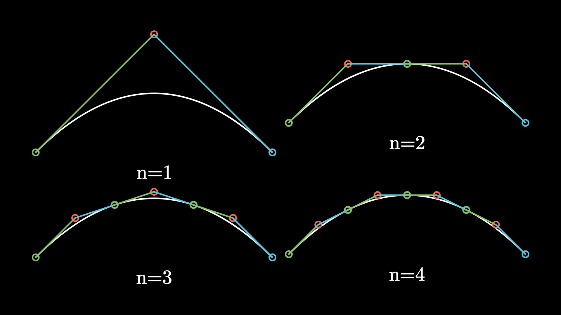

Parameters:

• points (BezierPointsLike) – The control points of the Bézier curve.

• n_divisions (int) – The number of curves to subdivide the Bézier curve into

Returns:

An array containing the points defining the new \(n\) subcurves.

Return type:

Spline